
Working with color
Color images are typically represented using several ‘color planes.’ For example, an RGB color image contains a red color plane, a green color plane, and a blue color plane. When overlaid and mixed, the three planes make up the full color image. To compress a color image, the still image compression techniques described earlier can be applied to each color plane in turn.
Imaging and video applications often use a color scheme in which the color planes do not correspond to specific colors; instead, one color plane contains luminance information (the overall brightness of each pixel in the color image), and two more color planes contain color (chrominance) information that when combined with luminance can be used to derive the specific levels of the red, green and blue components of each image pixel.
Such a color scheme is convenient because the human eye is more sensitive to luminance than to color, so the chrominance planes can often be stored and/ or encoded at a lower image resolution than the luminance information. Specifically, video compression algorithms typically encode the chrominance planes with half the horizontal resolution and half the vertical resolution of the luminance plane. Thus, for every 16-pixel by 16-pixel region in the luminance plane, each chrominance plane contains one 8-pixel by 8-pixel block. In typical video compression algorithms, a ‘macro block’ is a 16×16 region in the video frame that contains four 8×8 luminance blocks and the two corresponding 8×8 chrominance blocks.
Adding motion to the mix
Video compression algorithms share many of the compression techniques used in still image compression. A key difference, however, is that video compression can take advantage of the similarities between successive video frames to achieve even better compression ratios. Using the techniques described earlier, still-image compression algorithms such as JPEG can achieve good image quality at a compression ratio of about 10:1. The most advanced still image codecs may achieve good image quality at compression ratios as high as 30:1. In contrast, video compression algorithms can provide good video quality at ratios of up to 200:1. This increased efficiency is accomplished with the addition of video specific compression techniques such as motion estimation and motion compensation.
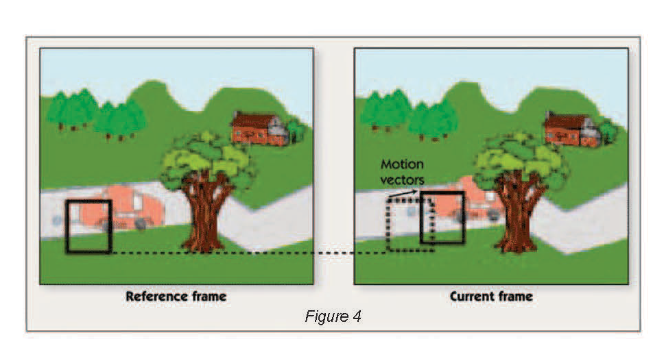
For each macro block in the current frame, motion estimation attempts to find a region in a previously encoded frame (called a ‘reference frame’) that is a close match. The spatial offset between the current block and selected block from the reference frame is called a ‘motion vector,’ as shown in figure 4. The encoder computes the pixel-by-pixel difference between the selected block from the reference frame and the current block, and transmits this ‘prediction error’ along with the motion vector. Most video compression standards allow motion-based prediction to be bypassed if the encoder fails to find a good match for the macro block. In this case, the macro block itself is encoded instead of the prediction error.
Motion estimation predicts the contents of each macro block based on motion relative to a reference frame. The ref erence frame is searched to find the 16×16 block that matches the macro block; motion vectors are encoded, and the difference between predicted and actual macro block pixels is encoded in the current frame.
Note that the reference frame isn’t always the previously displayed frame in the sequence of video frames. Video compression algorithms commonly encode frames in a different order from the order in which they are displayed. The encoder may skip several frames ahead and encode a future video frame, then skip backward and encode the next frame in the display sequence. This is done so that motion estimation can be performed backward in time, using the encoded future frame as a reference frame. Video compression algorithms also commonly allow the use of two reference frames – one previously displayed frame and one previously encoded future frame.
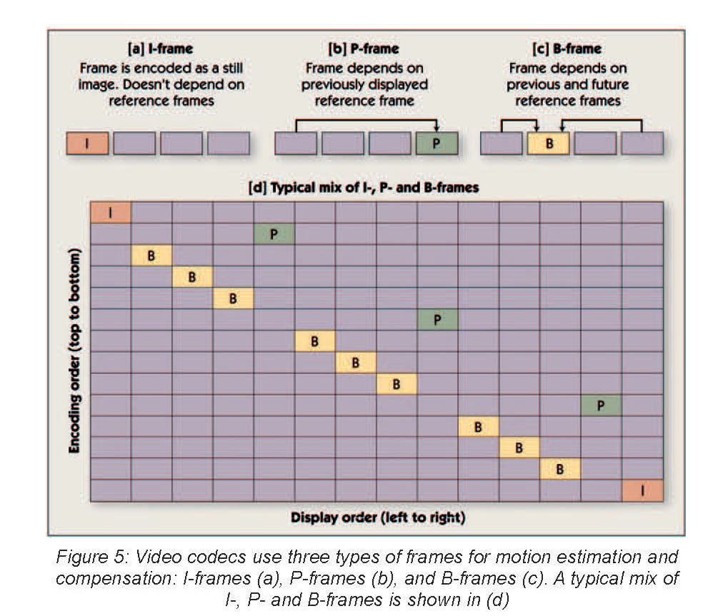
Video compression algorithms periodically encode one video frame using still-image coding techniques only, without relying on previously encoded frames. These frames are called ‘intra frames’ or ‘I-frames.’ If a frame in the compressed bit stream is corrupted by errors, the video decoder can ‘restart’ at the next I-frame, which doesn’t require a reference frame for reconstruction.
As shown in Figure 5, frames that are encoded using only a previously displayed reference frame are called ‘P-frames,’ and frames that are encoded using both future and previously displayed reference frames are called ‘B-frames.’ A typical sequence of frames is illustrated in Figure 5[d].
One factor that complicates motion estimation is that the displacement of an object from the reference frame to the current frame may be a non-integer number of pixels. For example, suppose that an object has moved 22.5 pixels to the right and 17.25 pixels upward. To handle such situations, modern video compression standards allow motion vectors to have non-integer values – motion vector resolutions of one-half or one-quarter of a pixel are common. To support searching for block matches at partial-pixel displacements, the encoder must use interpolation to estimate the reference frame’s pixel values at non-integer locations.
The simplest and most thorough way to perform motion estimation is to evaluate every possible 16×16 region in the search area, and select the best match. Typically, a ‘sum of absolute differences’ (SAD) or ‘sum of squared differences’ (SSD) computation is used to determine how closely a candidate 16×16 region matches a macro block. The SAD or SSD is often computed for the luminance plane only, but can also include the chrominance planes. But this approach can be overly demanding on processors – exhaustively searching an area of 48×24 pixels requires over 8 billion arithmetic operations per second at QVGA (640×480) video resolution and a frame rate of 30 frames per second.
Because of this high computational load, practical implementations of motion estimation do not use an exhaustive search. Instead, motion estimation algorithms use various methods to select a limited number of promising candidate motion vectors (roughly 10 to 100 vectors in most cases) and evaluate only 16×16 regions corresponding to these candidate vectors. One approach is to select the candidate motion vectors in several stages. For example, five initial candidate vectors may be selected and evaluated. The results are used to eliminate unlikely portions of the search area and zero in on the most promising portion of the search area. Five new vectors are selected and the process is repeated. After a few such stages, the best motion vector found so far is selected.
Another approach analyzes the motion vectors previously selected for surrounding macro blocks in the current and previous frames in an effort to predict the motion in the current macro block. A handful of candidate motion vectors are selected based on this analysis, and only those vectors are evaluated.
By selecting a small number of candidate vectors instead of scanning the search area exhaustively, the computational demand of motion estimation can be reduced considerably – sometimes by over two orders of magnitude. But there is a trade-off between processing load and image quality or compression efficiency. In general, searching a larger number of candidate motion vectors allows the encoder to find a block in the reference frame that better matches each block in the current frame, thus reducing the prediction error. The lower the predication error, the fewer are the bits that are needed to encode the image. So increasing the number of candidate vectors allows a reduction in compressed bit rate, at the cost of performing more SAD (or SSD) computations. Or, alternatively, increasing the number of candidate vectors while holding the compressed bit rate constant allows the prediction error to be encoded with higher precision, improving image quality.
Some codecs (including H.264) allow a 16×16 macro block to be subdivided into smaller blocks (e.g., various combinations of 8×8, 4×8, 8×4 and 4×4 blocks) to lower the prediction error. Each of these smaller blocks can have its own motion vector. The motion estimation search for such a scheme begins by finding a good position for the entire 16×16 block. If the match is close enough, there’s no need to subdivide further. But if the match is poor, then the algorithm starts at the best position found so far, and further subdivides the original block into 8×8 blocks. For each 8×8 block, the algorithm searches for the best position near the position selected by the 16×16 search. Depending on how quickly a good match is found, the algorithm can continue the process using smaller blocks of 8×4, 4×8 etc.
Even with drastic reductions in the number of candidate motion vectors, motion estimation is the most computationally demanding task in video compression applications. The inclusion of motion estimation makes video encoding much more computationally demanding than decoding. Motion estimation can require as much as 80% of the processor cycles spent in the video encoder. Therefore, many processors targeting multimedia applications provide a specialized instruction to accelerate SAD computations or a dedicated SAD co-processor to offload this task from the CPU. For example, ARM’s ARM11 core provides an instruction to accelerate SAD computation, and some members of Texas Instruments’ TMS320C55x family of DSPs provide an SAD co-processor.
Note that in order to perform motion estimation, the encoder must keep one or two reference frames in memory in addition to the current frame. The required frame buffers are very often larger than the available on-chip memory, requiring additional memory chips in many applications. Keeping reference frames in off-chip memory results in very high external memory bandwidth in the encoder, although large on-chip caches can help reduce the required bandwidth considerably.
<- Previous | 1 | 2 | 3 | 4 | Next ->